Injective Function (One-to-One Function)
Provided that $s(A) \leq s(B)$,
let $f: A \to B$ be a given function. If every distinct element in the domain $A$ maps to a distinct element in the codomain $B$, then this function is called an injective function.
That is, for $y = f(x)$,
\[
x_1 \neq x_2 \Rightarrow f(x_1) \neq f(x_2)
\]
or equivalently,
\[
f(x_1) = f(x_2) \Rightarrow x_1 = x_2 \]
Examples:
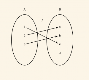
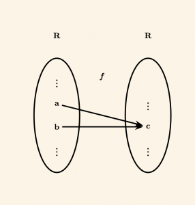
$\bullet \quad f: A \to B$ is injective because every element in $A$ maps to a distinct image in $B$. Furthermore, since there are unmapped elements remaining in the codomain $B$, it is injective and into (non-surjective).
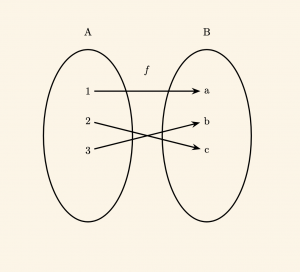
$\bullet \quad f: A \to B$ is a bijective function, meaning it is both injective (one-to-one) and surjective (onto).
$\bullet \quad f: \mathbb{N} \to \mathbb{Z}$, defined by $f(x) = 2x^3 – 7$:
\[
f(x_1) = 2x_1^3 – 7 \quad \text{and} \quad f(x_2) = 2x_2^3 – 7
\]
\[
f(x_1) = f(x_2) \Rightarrow 2x_1^3 – 7 = 2x_2^3 – 7
\]
\[
\Rightarrow x_1 = x_2 \quad \text{Therefore, the function is injective.}
\]
$\bullet \quad f: \mathbb{R} \to \mathbb{R}$, defined by $f(x) = 2x^2 + 1$:
\[
f(x_1) = 2x_1^2 + 1 \quad \text{and} \quad f(x_2) = 2x_2^2 + 1
\]
\[
f(x_1) = f(x_2) \Rightarrow 2x_1^2 + 1 = 2x_2^2 + 1
\]
\[
\Rightarrow x_1^2 = x_2^2 \Rightarrow x_1 = \pm x_2
\]
Since distinct inputs can yield identical outputs, the function is not injective.
$\bullet \quad f: \mathbb{N} \to \mathbb{N}$, defined by $f(x) = x^2 + x + 1$:
\[
f(x_1) = x_1^2 + x_1 + 1 \quad \text{and} \quad f(x_2) = x_2^2 + x_2 + 1
\]
\[
f(x_1) = f(x_2) \Rightarrow x_1^2 + x_1 + 1 = x_2^2 + x_2 + 1
\]
\[
\Rightarrow x_1^2 – x_2^2 + x_1 – x_2 = 0
\]
\[
\Rightarrow (x_1 – x_2)(x_1 + x_2 + 1) = 0
\]
Since $x \in \mathbb{N}$, the term $x_1 + x_2 + 1 \neq 0$. Thus, it follows that:
\[
x_1 – x_2 = 0 \Rightarrow x_1 = x_2
\]
Consequently, the function is injective.
$\bullet \quad f: \mathbb{R} – \{-1\} \to \mathbb{R} – \{2\}$, defined by
\[
f(x) = \frac{2x – 1}{x + 1}
\]
Setting up the equation:
\[
f(x_1) = \frac{2x_1 – 1}{x_1 + 1} \quad \text{and} \quad f(x_2) = \frac{2x_2 – 1}{x_2 + 1}
\]
Using cross-multiplication:
\[
f(x_1) = f(x_2) \Rightarrow \frac{2x_1 – 1}{x_1 + 1} = \frac{2x_2 – 1}{x_2 + 1}
\]
\[
\Rightarrow 2x_1 x_2 – x_2 + 2x_1 – 1 = 2x_1 x_2 – x_1 + 2x_2 – 1
\]
\[
\Rightarrow 3x_1 = 3x_2 \Rightarrow x_1 = x_2
\]
Therefore, the function is injective.
The Horizontal Line Test:
To determine the properties of a graphically defined function $y = f(x)$, construct horizontal lines through points along the codomain across the $y$-axis:
1) If any horizontal line fails to intersect the graph, the function is into (non-surjective).
2) If every horizontal line intersects the graph at least once, the function is surjective (onto).
3) If every horizontal line intersects the graph at most at one point, the function is injective (one-to-one).
Example:
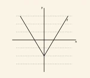
The graph of a function $f: \mathbb{R} \to \mathbb{R}$ is shown.
Since the codomain consists of all real numbers, we evaluate horizontal lines passing through the $y$-axis. Because there are lines that do not intersect the graph at all, it is an into function. Furthermore, because certain lines intersect the graph at multiple (two) points, it is not injective.
Geometrically, lines that do not intersect the curve signify unmapped elements within the codomain. Lines intersecting the curve multiple times indicate that more than one element in the domain maps to the same output.
Further Examples:
Let us classify the properties of the following functions based on the horizontal line test.
1)
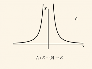
The function $f_1$ is not injective because horizontal lines cross the curve at two points. However, since every horizontal line intersects the graph at least once, it is surjective.
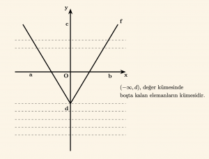
2)
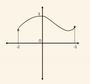 The function $f_2$ is not injective because certain horizontal lines intersect the graph multiple times. Additionally, because there are horizontal lines that do not intersect the curve at all, it is an into function.
3)
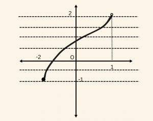
The function $f_3$ is surjective since there are no horizontal lines that fail to intersect the graph. Furthermore, because no horizontal line cuts the graph at more than one point, it is also injective. Thus, it is bijective.
Counting Injective Functions:
Let $s(A) = m$ and $s(B) = n$. The total number of unique injective functions that can be defined from $A$ to $B$ is given by the permutation formula:
\[
P(n, m) = \frac{n!}{(n – m)!} \quad (\text{where } n \geq m)
\]
For a function $f: A \to B$ to be both injective and surjective (bijective), the conditions require $s(A) = s(B) = n$. Therefore:
The total number of bijective functions from $A$ to $B$ is:
\[
\frac{n!}{(n – n)!} = n!
\]
Example:
Given $A = \{ 1, 2, 3 \}$ and $B = \{ a, b, c, d \}$,
the total number of injective functions $f: A \to B$ is:
\[
\frac{4!}{(4 – 3)!} = 24
\]
The total number of bijective functions $f: A \to A$ is:
\[
3! = 6
\]
← Previous Page | Next Page →