Graphing a System of Inequalities

 

The set of points in the coordinate plane that simultaneously satisfy all the inequalities in a given system is called the graph of the system of inequalities.

To plot the graph of a system of inequalities, the individual graph of each inequality within the system is sketched on the same coordinate axes.

The region where these graphs overlap (their intersection) defines the solution graph of the system of inequalities.

 

Example:

 

\[
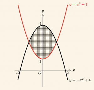
\left.
\begin{aligned}
y \geq x^2 + 1\\
\\
y + x^2 – 4 < 0\\
\end{aligned}
\right\} \Rightarrow \quad \text{Let us sketch the graph of this system of inequalities.}
\]

 

\[
\left.
\begin{aligned}
y \geq x^2 + 1 \\
\\
y +x^2 – 4 < 0\\
\end{aligned}
\right\} \Rightarrow \left. \begin{aligned} y \geq x^2 + 1 \\ \\ y < -x^2 + 4 \\ \end{aligned} \right\}
\]

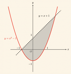
Example:

 

\[
\left.
\begin{aligned}
y \geq x^2 – 1\\
\\
y < x + 1 \\
\end{aligned}
\right\} \Rightarrow \quad \text{Let us sketch the graph of this system of inequalities.}
\]

 

 

Note:

 

The solution set of a combined inequality system of the form \( f(x) < y < g(x) \) corresponds to the geometric region bounded between the curves (or lines) \( y = f(x) \) and \( y = g(x) \).

 

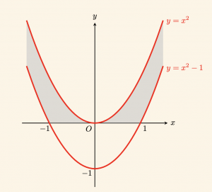
Example:

 

\[
\left.
\begin{aligned}
x^2 – 1 \leq y \leq x^2 \\
\\
y \geq 0 \\
\end{aligned}
\right\} \Rightarrow \quad \text{Let us sketch the graph of this system of inequalities.}
\]

This system establishes the following constraints:

\(\bullet \) \(\quad\) The region is restricted by \( y \geq 0 \), meaning only the upper half-plane is considered.
\(\bullet \quad\) The vertical range is bounded from below by the lower limit \( y = x^2 – 1 \) and from above by the upper limit \( y = x^2 \).

Thus, the shaded area represents the common solution region satisfying the conditions:
\[
x^2 – 1 \leq y \leq x^2 \quad \text{and} \quad y \geq 0
\]
The resulting parabolic band region is displayed exclusively where \( y \geq 0 \).

 

 

 

← Previous Page | Next Page →